This is an automated email from the ASF dual-hosted git repository.

caogaofei pushed a commit to branch main
in repository https://gitbox.apache.org/repos/asf/iotdb-docs.git
The following commit(s) were added to refs/heads/main by this push:
new ca450c8 AINode analysis
ca450c8 is described below
commit ca450c8e7571665ef23acb2bcd4608fbdd8e2d60
Author: W1y1r <[email protected]>
AuthorDate: Thu Sep 26 12:22:24 2024 +0800
AINode analysis
---
src/UserGuide/Master/User-Manual/AINode_timecho.md | 52 +++++++++++-----------
src/UserGuide/latest/User-Manual/AINode_timecho.md | 52 +++++++++++-----------
.../UserGuide/Master/User-Manual/AINode_timecho.md | 52 ++++++++++------------
.../UserGuide/latest/User-Manual/AINode_timecho.md | 51 ++++++++++-----------
4 files changed, 98 insertions(+), 109 deletions(-)
diff --git a/src/UserGuide/Master/User-Manual/AINode_timecho.md
b/src/UserGuide/Master/User-Manual/AINode_timecho.md
index ac19101..5b6b691 100644
--- a/src/UserGuide/Master/User-Manual/AINode_timecho.md
+++ b/src/UserGuide/Master/User-Manual/AINode_timecho.md
@@ -405,7 +405,8 @@ Total line number = 48
#### Example of using the count window function
-This window is mainly used for computational tasks, when the model
corresponding to the task can only process a fixed row of data at a time and
what is ultimately desired is indeed multiple sets of predictions, using this
window function allows for sequential inference using a sliding window of
points. Suppose we now have an anomaly detection model anomaly_example(input:
[24,2], output[1,1]) that generates a 0/1 label for each row of data, an
example of its use is shown below:
+This window is mainly used for computational tasks. When the task's
corresponding model can only handle a fixed number of rows of data at a time,
but the final desired outcome is multiple sets of prediction results, this
window function can be used to perform continuous inference using a sliding
window of points. Suppose we now have an anomaly detection model
`anomaly_example(input: [24,2], output[1,1])`, which generates a 0/1 label for
every 24 rows of data. An example of its use is as [...]
+
```Shell
IoTDB> select s1,s2 from root.**
+-----------------------------+-------------------+-------------------+
@@ -441,7 +442,7 @@ IoTDB> call inference(anomaly_example,"select s0,s1 from
root.**",window=count(2
Total line number = 4
```
-where the labels of each row in the result set correspond to the model output
corresponding to the 16 rows of input.
+In the result set, each row's label corresponds to the output of the anomaly
detection model after inputting each group of 24 rows of data.
## Privilege Management
@@ -519,9 +520,9 @@ Total line number = 48
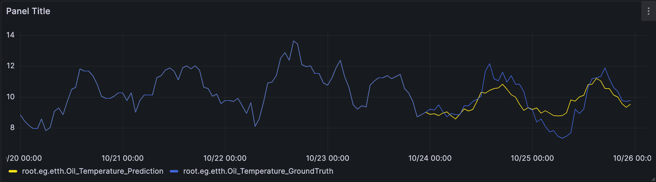
We compare the results of the prediction of the oil temperature with the real
results, and we can get the following image.
-The data before 10/24 00:00 in the image is the past data input into the
model, the yellow line after 10/24 00:00 is the prediction of oil temperature
given by the model, and the blue colour is the actual oil temperature data in
the dataset (used for comparison).
+The data before 10/24 00:00 represents the past data input to the model, the
blue line after 10/24 00:00 is the oil temperature forecast result given by the
model, and the red line is the actual oil temperature data from the dataset
(used for comparison).
-
+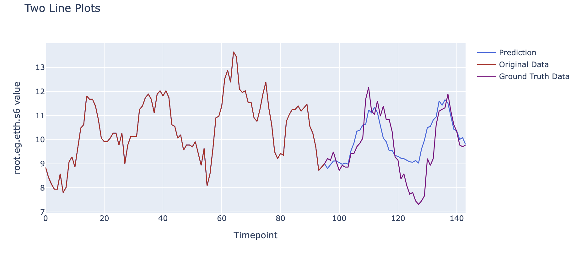
As can be seen, we have used the relationship between the six load information
and the corresponding time oil temperatures for the past 96 hours (4 days) to
model the possible changes in this data for the oil temperature for the next 48
hours (2 days) based on the inter-relationships between the sequences learned
previously, and it can be seen that the predicted curves maintain a high degree
of consistency in trend with the actual results after visualisation.
@@ -545,13 +546,9 @@ bash ./import-csv.sh -h 127.0.0.1 -p 6667 -u root -pw root
-f ... /... /data.csv
#### Step 2: Model Import
-We can enter the following SQL in iotdb-cli to pull a trained model from
huggingface for registration for subsequent inference.
-
-```SQL
-create model patchtst using uri
`https://huggingface.co/hvlgo/patchtst/resolve/main`
-```
+We can select built-in models or registered models in IoTDB CLI for subsequent
inference.
-We use the deep model PatchTST for prediction, which is a transformer-based
temporal prediction model with excellent performance in long time series
prediction tasks.
+We use the built-in model STLForecaster for prediction. STLForecaster is a
time series forecasting method based on the STL implementation in the
statsmodels library.
#### Step 3: Model Inference
@@ -560,39 +557,40 @@ IoTDB> select * from root.eg.voltage limit 96
+-----------------------------+------------------+------------------+------------------+
|
Time|root.eg.voltage.s0|root.eg.voltage.s1|root.eg.voltage.s2|
+-----------------------------+------------------+------------------+------------------+
-|2024-03-15T20:35:31.000+08:00| 2037.0| 2017.0|
2032.0|
-|2024-03-15T20:35:37.000+08:00| 2015.0| 2014.0|
2019.0|
-|2024-03-15T20:35:44.000+08:00| 2014.0| 2007.0|
2019.0|
+|2023-02-14T20:38:32.000+08:00| 2038.0| 2028.0|
2041.0|
+|2023-02-14T20:38:38.000+08:00| 2014.0| 2005.0|
2018.0|
+|2023-02-14T20:38:44.000+08:00| 2014.0| 2005.0|
2018.0|
......
-|2024-03-15T20:43:51.000+08:00| 2024.0| 2012.0|
2022.0|
-|2024-03-15T20:43:56.000+08:00| 2023.0| 2016.0|
2022.0|
-|2024-03-15T20:44:03.000+08:00| 2024.0| 2016.0|
2022.0|
+|2023-02-14T20:47:52.000+08:00| 2024.0| 2016.0|
2027.0|
+|2023-02-14T20:47:57.000+08:00| 2024.0| 2016.0|
2027.0|
+|2023-02-14T20:48:03.000+08:00| 2024.0| 2016.0|
2027.0|
+-----------------------------+------------------+------------------+------------------+
Total line number = 96
-IoTDB> call inference(patchtst, "select s0,s1,s2 from root.eg.voltage",
window=head(96))
+IoTDB> call inference(_STLForecaster, "select s0,s1,s2 from root.eg.voltage",
window=head(96),predict_length=48)
+---------+---------+---------+
| output0| output1| output2|
+---------+---------+---------+
-|2013.4113|2011.2539|2010.2732|
-|2013.2792| 2007.902|2035.7709|
-|2019.9114|2011.0453|2016.5848|
+|2026.3601|2018.2953|2029.4257|
+|2019.1538|2011.4361|2022.0888|
+|2025.5074|2017.4522|2028.5199|
......
-|2018.7078|2009.7993|2017.3502|
-|2033.9062|2010.2087|2018.1757|
-|2022.2194| 2011.923|2020.5442|
-|2022.1393|2023.4688|2020.9344|
+
+|2022.2336|2015.0290|2025.1023|
+|2015.7241|2008.8975|2018.5085|
+|2022.0777|2014.9136|2024.9396|
+|2015.5682|2008.7821|2018.3458|
+---------+---------+---------+
Total line number = 48
```
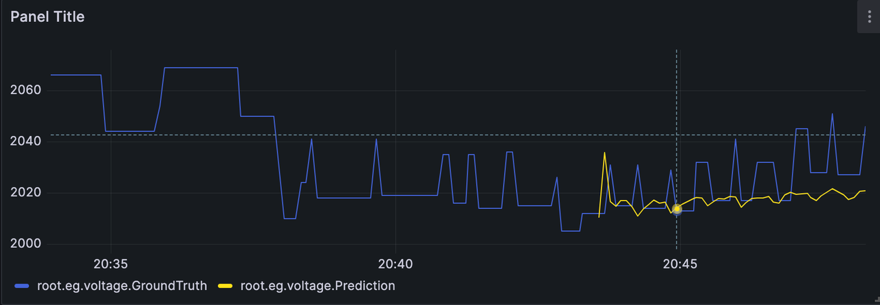
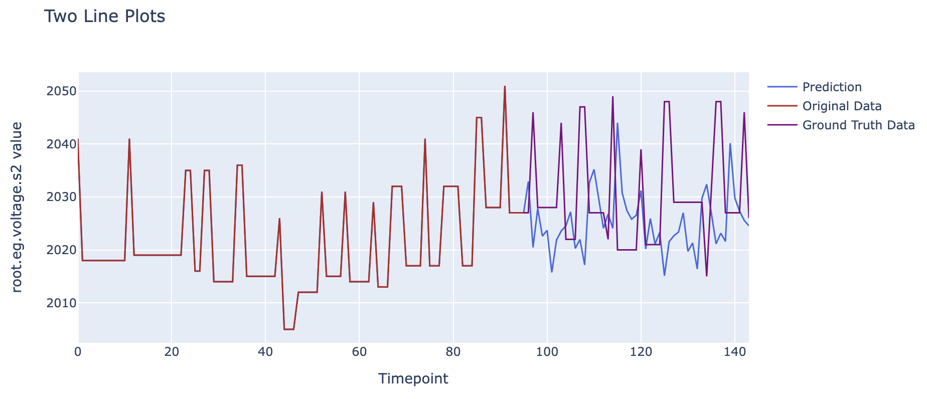
Comparing the predicted results of the C-phase voltage with the real results,
we can get the following image.
-The data before 02/14 20:44 is the past data input to the model, the yellow
line after 02/14 20:44 is the predicted C-phase voltage given by the model, and
the blue colour is the actual A-phase voltage data in the dataset (used for
comparison).
+The data before 02/14 20:48 represents the past data input to the model, the
blue line after 02/14 20:48 is the predicted result of phase C voltage given by
the model, while the red line is the actual phase C voltage data from the
dataset (used for comparison).
-
+
-It can be seen that we have used the data of the last 8 minutes of voltage to
model the possible changes in the A-phase voltage for the next 4 minutes based
on the inter-relationships between the sequences learned earlier, and it can be
seen that the predicted curves and the actual results maintain a high degree of
synchronicity in terms of trends after visualisation.
+It can be seen that we used the voltage data from the past 10 minutes and,
based on the previously learned inter-sequence relationships, modeled the
possible changes in the phase C voltage data for the next 5 minutes. The
visualized forecast curve shows a certain degree of synchronicity with the
actual results in terms of trend.
### Anomaly Detection
diff --git a/src/UserGuide/latest/User-Manual/AINode_timecho.md
b/src/UserGuide/latest/User-Manual/AINode_timecho.md
index 0177505..4291584 100644
--- a/src/UserGuide/latest/User-Manual/AINode_timecho.md
+++ b/src/UserGuide/latest/User-Manual/AINode_timecho.md
@@ -406,7 +406,8 @@ Total line number = 48
#### Example of using the count window function
-This window is mainly used for computational tasks, when the model
corresponding to the task can only process a fixed row of data at a time and
what is ultimately desired is indeed multiple sets of predictions, using this
window function allows for sequential inference using a sliding window of
points. Suppose we now have an anomaly detection model anomaly_example(input:
[24,2], output[1,1]) that generates a 0/1 label for each row of data, an
example of its use is shown below:
+This window is mainly used for computational tasks. When the task's
corresponding model can only handle a fixed number of rows of data at a time,
but the final desired outcome is multiple sets of prediction results, this
window function can be used to perform continuous inference using a sliding
window of points. Suppose we now have an anomaly detection model
`anomaly_example(input: [24,2], output[1,1])`, which generates a 0/1 label for
every 24 rows of data. An example of its use is as [...]
+
```Shell
IoTDB> select s1,s2 from root.**
+-----------------------------+-------------------+-------------------+
@@ -442,7 +443,7 @@ IoTDB> call inference(anomaly_example,"select s0,s1 from
root.**",window=count(2
Total line number = 4
```
-where the labels of each row in the result set correspond to the model output
corresponding to the 16 rows of input.
+In the result set, each row's label corresponds to the output of the anomaly
detection model after inputting each group of 24 rows of data.
## Privilege Management
@@ -520,9 +521,9 @@ Total line number = 48
We compare the results of the prediction of the oil temperature with the real
results, and we can get the following image.
-The data before 10/24 00:00 in the image is the past data input into the
model, the yellow line after 10/24 00:00 is the prediction of oil temperature
given by the model, and the blue colour is the actual oil temperature data in
the dataset (used for comparison).
+The data before 10/24 00:00 represents the past data input to the model, the
blue line after 10/24 00:00 is the oil temperature forecast result given by the
model, and the red line is the actual oil temperature data from the dataset
(used for comparison).
-
+
As can be seen, we have used the relationship between the six load information
and the corresponding time oil temperatures for the past 96 hours (4 days) to
model the possible changes in this data for the oil temperature for the next 48
hours (2 days) based on the inter-relationships between the sequences learned
previously, and it can be seen that the predicted curves maintain a high degree
of consistency in trend with the actual results after visualisation.
@@ -546,13 +547,9 @@ bash ./import-csv.sh -h 127.0.0.1 -p 6667 -u root -pw root
-f ... /... /data.csv
#### Step 2: Model Import
-We can enter the following SQL in iotdb-cli to pull a trained model from
huggingface for registration for subsequent inference.
-
-```SQL
-create model patchtst using uri
`https://huggingface.co/hvlgo/patchtst/resolve/main`
-```
+We can select built-in models or registered models in IoTDB CLI for subsequent
inference.
-We use the deep model PatchTST for prediction, which is a transformer-based
temporal prediction model with excellent performance in long time series
prediction tasks.
+We use the built-in model STLForecaster for prediction. STLForecaster is a
time series forecasting method based on the STL implementation in the
statsmodels library.
#### Step 3: Model Inference
@@ -561,39 +558,40 @@ IoTDB> select * from root.eg.voltage limit 96
+-----------------------------+------------------+------------------+------------------+
|
Time|root.eg.voltage.s0|root.eg.voltage.s1|root.eg.voltage.s2|
+-----------------------------+------------------+------------------+------------------+
-|2024-03-15T20:35:31.000+08:00| 2037.0| 2017.0|
2032.0|
-|2024-03-15T20:35:37.000+08:00| 2015.0| 2014.0|
2019.0|
-|2024-03-15T20:35:44.000+08:00| 2014.0| 2007.0|
2019.0|
+|2023-02-14T20:38:32.000+08:00| 2038.0| 2028.0|
2041.0|
+|2023-02-14T20:38:38.000+08:00| 2014.0| 2005.0|
2018.0|
+|2023-02-14T20:38:44.000+08:00| 2014.0| 2005.0|
2018.0|
......
-|2024-03-15T20:43:51.000+08:00| 2024.0| 2012.0|
2022.0|
-|2024-03-15T20:43:56.000+08:00| 2023.0| 2016.0|
2022.0|
-|2024-03-15T20:44:03.000+08:00| 2024.0| 2016.0|
2022.0|
+|2023-02-14T20:47:52.000+08:00| 2024.0| 2016.0|
2027.0|
+|2023-02-14T20:47:57.000+08:00| 2024.0| 2016.0|
2027.0|
+|2023-02-14T20:48:03.000+08:00| 2024.0| 2016.0|
2027.0|
+-----------------------------+------------------+------------------+------------------+
Total line number = 96
-IoTDB> call inference(patchtst, "select s0,s1,s2 from root.eg.voltage",
window=head(96))
+IoTDB> call inference(_STLForecaster, "select s0,s1,s2 from root.eg.voltage",
window=head(96),predict_length=48)
+---------+---------+---------+
| output0| output1| output2|
+---------+---------+---------+
-|2013.4113|2011.2539|2010.2732|
-|2013.2792| 2007.902|2035.7709|
-|2019.9114|2011.0453|2016.5848|
+|2026.3601|2018.2953|2029.4257|
+|2019.1538|2011.4361|2022.0888|
+|2025.5074|2017.4522|2028.5199|
......
-|2018.7078|2009.7993|2017.3502|
-|2033.9062|2010.2087|2018.1757|
-|2022.2194| 2011.923|2020.5442|
-|2022.1393|2023.4688|2020.9344|
+
+|2022.2336|2015.0290|2025.1023|
+|2015.7241|2008.8975|2018.5085|
+|2022.0777|2014.9136|2024.9396|
+|2015.5682|2008.7821|2018.3458|
+---------+---------+---------+
Total line number = 48
```
Comparing the predicted results of the C-phase voltage with the real results,
we can get the following image.
-The data before 02/14 20:44 is the past data input to the model, the yellow
line after 02/14 20:44 is the predicted C-phase voltage given by the model, and
the blue colour is the actual A-phase voltage data in the dataset (used for
comparison).
+The data before 02/14 20:48 represents the past data input to the model, the
blue line after 02/14 20:48 is the predicted result of phase C voltage given by
the model, while the red line is the actual phase C voltage data from the
dataset (used for comparison).
-
+
-It can be seen that we have used the data of the last 8 minutes of voltage to
model the possible changes in the A-phase voltage for the next 4 minutes based
on the inter-relationships between the sequences learned earlier, and it can be
seen that the predicted curves and the actual results maintain a high degree of
synchronicity in terms of trends after visualisation.
+It can be seen that we used the voltage data from the past 10 minutes and,
based on the previously learned inter-sequence relationships, modeled the
possible changes in the phase C voltage data for the next 5 minutes. The
visualized forecast curve shows a certain degree of synchronicity with the
actual results in terms of trend.
### Anomaly Detection
diff --git a/src/zh/UserGuide/Master/User-Manual/AINode_timecho.md
b/src/zh/UserGuide/Master/User-Manual/AINode_timecho.md
index 42b9254..0589092 100644
--- a/src/zh/UserGuide/Master/User-Manual/AINode_timecho.md
+++ b/src/zh/UserGuide/Master/User-Manual/AINode_timecho.md
@@ -402,7 +402,7 @@ Total line number = 48
#### 使用count窗口函数的示例
-该窗口主要用于计算式任务,当任务对应的模型一次只能处理固定行数据而最终想要的确实多组预测结果时,使用该窗口函数可以使用点数滑动窗口进行连续推理。假设我们现在有一个异常检测模型anomaly_example(input:
[24,2], output[1,1]),对每行数据会生成一个0/1的标签,其使用示例如下:
+该窗口主要用于计算式任务,当任务对应的模型一次只能处理固定行数据而最终想要的确实多组预测结果时,使用该窗口函数可以使用点数滑动窗口进行连续推理。假设我们现在有一个异常检测模型anomaly_example(input:
[24,2], output[1,1]),对每24行数据会生成一个0/1的标签,其使用示例如下:
```Shell
IoTDB> select s1,s2 from root.**
@@ -439,7 +439,7 @@ IoTDB> call inference(anomaly_example,"select s0,s1 from
root.**",window=count(2
Total line number = 4
```
-其中结果集中的每行的标签对应16行输入对应的模型输出。
+其中结果集中每行的标签对应每24行数据为一组,输入该异常检测模型后的输出。
## 权限管理
@@ -517,9 +517,9 @@ Total line number = 48
我们将对油温的预测的结果和真实结果进行对比,可以得到以下的图像。
-图中10/24 00:00之前的数据为输入模型的过去数据,10/24
00:00后的黄色线条为模型给出的油温预测结果,而蓝色为数据集中实际的油温数据(用于进行对比)。
+图中10/24 00:00之前的数据为输入模型的过去数据,10/24
00:00后的蓝色线条为模型给出的油温预测结果,而红色为数据集中实际的油温数据(用于进行对比)。
-
+
可以看到,我们使用了过去96个小时(4天)的六个负载信息和对应时间油温的关系,基于之前学习到的序列间相互关系对未来48个小时(2天)的油温这一数据的可能变化进行了建模,可以看到可视化后预测曲线与实际结果在趋势上保持了较高程度的一致性。
@@ -543,54 +543,50 @@ bash ./import-csv.sh -h 127.0.0.1 -p 6667 -u root -pw
root -f ../../data.csv
#### 步骤二:模型导入
-我们可以在iotdb-cli 中输入以下SQL从 huggingface 上拉取一个已经训练好的模型进行注册,用于后续的推理。
-
-```SQL
-create model patchtst using uri
'https://huggingface.co/hvlgo/patchtst/resolve/main'
-```
+我们可以在iotdb-cli 中选择内置模型或已经注册好的模型用于后续的推理。
-我们采用深度模型PatchTST进行预测,PatchTST 是一种基于 transformer 的时序预测模型,在长时间序列预测任务中有出色的表现。
+我们采用内置模型STLForecaster进行预测,STLForecaster 是一个基于 statsmodels 库中 STL 实现的时间序列预测方法。
#### 步骤三:模型推理
-
```Shell
IoTDB> select * from root.eg.voltage limit 96
+-----------------------------+------------------+------------------+------------------+
|
Time|root.eg.voltage.s0|root.eg.voltage.s1|root.eg.voltage.s2|
+-----------------------------+------------------+------------------+------------------+
-|2024-03-15T20:35:31.000+08:00| 2037.0| 2017.0|
2032.0|
-|2024-03-15T20:35:37.000+08:00| 2015.0| 2014.0|
2019.0|
-|2024-03-15T20:35:44.000+08:00| 2014.0| 2007.0|
2019.0|
+|2023-02-14T20:38:32.000+08:00| 2038.0| 2028.0|
2041.0|
+|2023-02-14T20:38:38.000+08:00| 2014.0| 2005.0|
2018.0|
+|2023-02-14T20:38:44.000+08:00| 2014.0| 2005.0|
2018.0|
......
-|2024-03-15T20:43:51.000+08:00| 2024.0| 2012.0|
2022.0|
-|2024-03-15T20:43:56.000+08:00| 2023.0| 2016.0|
2022.0|
-|2024-03-15T20:44:03.000+08:00| 2024.0| 2016.0|
2022.0|
+|2023-02-14T20:47:52.000+08:00| 2024.0| 2016.0|
2027.0|
+|2023-02-14T20:47:57.000+08:00| 2024.0| 2016.0|
2027.0|
+|2023-02-14T20:48:03.000+08:00| 2024.0| 2016.0|
2027.0|
+-----------------------------+------------------+------------------+------------------+
Total line number = 96
-IoTDB> call inference(patchtst, "select s0,s1,s2 from root.eg.voltage",
window=head(96))
+IoTDB> call inference(_STLForecaster, "select s0,s1,s2 from root.eg.voltage",
window=head(96),predict_length=48)
+---------+---------+---------+
| output0| output1| output2|
+---------+---------+---------+
-|2013.4113|2011.2539|2010.2732|
-|2013.2792| 2007.902|2035.7709|
-|2019.9114|2011.0453|2016.5848|
+|2026.3601|2018.2953|2029.4257|
+|2019.1538|2011.4361|2022.0888|
+|2025.5074|2017.4522|2028.5199|
......
-|2018.7078|2009.7993|2017.3502|
-|2033.9062|2010.2087|2018.1757|
-|2022.2194| 2011.923|2020.5442|
-|2022.1393|2023.4688|2020.9344|
+
+|2022.2336|2015.0290|2025.1023|
+|2015.7241|2008.8975|2018.5085|
+|2022.0777|2014.9136|2024.9396|
+|2015.5682|2008.7821|2018.3458|
+---------+---------+---------+
Total line number = 48
```
我们将对C相电压的预测的结果和真实结果进行对比,可以得到以下的图像。
-图中 02/14 20:44 之前的数据为输入模型的过去数据, 02/14 20:44
后的黄色线条为模型给出的C相电压预测结果,而蓝色为数据集中实际的A相电压数据(用于进行对比)。
+图中 02/14 20:48 之前的数据为输入模型的过去数据, 02/14 20:48
后的蓝色线条为模型给出的C相电压预测结果,而红色为数据集中实际的C相电压数据(用于进行对比)。
-
+
-可以看到,我们使用了过去8分钟的电压的数据,基于之前学习到的序列间相互关系对未来4分钟的A相电压这一数据的可能变化进行了建模,可以看到可视化后预测曲线与实际结果在趋势上保持了较高程度的同步性。
+可以看到,我们使用了过去10分钟的电压的数据,基于之前学习到的序列间相互关系对未来5分钟的C相电压这一数据的可能变化进行了建模,可以看到可视化后预测曲线与实际结果在趋势上保持了一定的同步性。
### 异常检测
diff --git a/src/zh/UserGuide/latest/User-Manual/AINode_timecho.md
b/src/zh/UserGuide/latest/User-Manual/AINode_timecho.md
index e5dad5c..0589092 100644
--- a/src/zh/UserGuide/latest/User-Manual/AINode_timecho.md
+++ b/src/zh/UserGuide/latest/User-Manual/AINode_timecho.md
@@ -402,7 +402,7 @@ Total line number = 48
#### 使用count窗口函数的示例
-该窗口主要用于计算式任务,当任务对应的模型一次只能处理固定行数据而最终想要的确实多组预测结果时,使用该窗口函数可以使用点数滑动窗口进行连续推理。假设我们现在有一个异常检测模型anomaly_example(input:
[24,2], output[1,1]),对每行数据会生成一个0/1的标签,其使用示例如下:
+该窗口主要用于计算式任务,当任务对应的模型一次只能处理固定行数据而最终想要的确实多组预测结果时,使用该窗口函数可以使用点数滑动窗口进行连续推理。假设我们现在有一个异常检测模型anomaly_example(input:
[24,2], output[1,1]),对每24行数据会生成一个0/1的标签,其使用示例如下:
```Shell
IoTDB> select s1,s2 from root.**
@@ -439,7 +439,7 @@ IoTDB> call inference(anomaly_example,"select s0,s1 from
root.**",window=count(2
Total line number = 4
```
-其中结果集中的每行的标签对应16行输入对应的模型输出。
+其中结果集中每行的标签对应每24行数据为一组,输入该异常检测模型后的输出。
## 权限管理
@@ -517,9 +517,9 @@ Total line number = 48
我们将对油温的预测的结果和真实结果进行对比,可以得到以下的图像。
-图中10/24 00:00之前的数据为输入模型的过去数据,10/24
00:00后的黄色线条为模型给出的油温预测结果,而蓝色为数据集中实际的油温数据(用于进行对比)。
+图中10/24 00:00之前的数据为输入模型的过去数据,10/24
00:00后的蓝色线条为模型给出的油温预测结果,而红色为数据集中实际的油温数据(用于进行对比)。
-
+
可以看到,我们使用了过去96个小时(4天)的六个负载信息和对应时间油温的关系,基于之前学习到的序列间相互关系对未来48个小时(2天)的油温这一数据的可能变化进行了建模,可以看到可视化后预测曲线与实际结果在趋势上保持了较高程度的一致性。
@@ -543,13 +543,9 @@ bash ./import-csv.sh -h 127.0.0.1 -p 6667 -u root -pw root
-f ../../data.csv
#### 步骤二:模型导入
-我们可以在iotdb-cli 中输入以下SQL从 huggingface 上拉取一个已经训练好的模型进行注册,用于后续的推理。
+我们可以在iotdb-cli 中选择内置模型或已经注册好的模型用于后续的推理。
-```SQL
-create model patchtst using uri
'https://huggingface.co/hvlgo/patchtst/resolve/main'
-```
-
-我们采用深度模型PatchTST进行预测,PatchTST 是一种基于 transformer 的时序预测模型,在长时间序列预测任务中有出色的表现。
+我们采用内置模型STLForecaster进行预测,STLForecaster 是一个基于 statsmodels 库中 STL 实现的时间序列预测方法。
#### 步骤三:模型推理
@@ -558,38 +554,39 @@ IoTDB> select * from root.eg.voltage limit 96
+-----------------------------+------------------+------------------+------------------+
|
Time|root.eg.voltage.s0|root.eg.voltage.s1|root.eg.voltage.s2|
+-----------------------------+------------------+------------------+------------------+
-|2024-03-15T20:35:31.000+08:00| 2037.0| 2017.0|
2032.0|
-|2024-03-15T20:35:37.000+08:00| 2015.0| 2014.0|
2019.0|
-|2024-03-15T20:35:44.000+08:00| 2014.0| 2007.0|
2019.0|
+|2023-02-14T20:38:32.000+08:00| 2038.0| 2028.0|
2041.0|
+|2023-02-14T20:38:38.000+08:00| 2014.0| 2005.0|
2018.0|
+|2023-02-14T20:38:44.000+08:00| 2014.0| 2005.0|
2018.0|
......
-|2024-03-15T20:43:51.000+08:00| 2024.0| 2012.0|
2022.0|
-|2024-03-15T20:43:56.000+08:00| 2023.0| 2016.0|
2022.0|
-|2024-03-15T20:44:03.000+08:00| 2024.0| 2016.0|
2022.0|
+|2023-02-14T20:47:52.000+08:00| 2024.0| 2016.0|
2027.0|
+|2023-02-14T20:47:57.000+08:00| 2024.0| 2016.0|
2027.0|
+|2023-02-14T20:48:03.000+08:00| 2024.0| 2016.0|
2027.0|
+-----------------------------+------------------+------------------+------------------+
Total line number = 96
-IoTDB> call inference(patchtst, "select s0,s1,s2 from root.eg.voltage",
window=head(96))
+IoTDB> call inference(_STLForecaster, "select s0,s1,s2 from root.eg.voltage",
window=head(96),predict_length=48)
+---------+---------+---------+
| output0| output1| output2|
+---------+---------+---------+
-|2013.4113|2011.2539|2010.2732|
-|2013.2792| 2007.902|2035.7709|
-|2019.9114|2011.0453|2016.5848|
+|2026.3601|2018.2953|2029.4257|
+|2019.1538|2011.4361|2022.0888|
+|2025.5074|2017.4522|2028.5199|
......
-|2018.7078|2009.7993|2017.3502|
-|2033.9062|2010.2087|2018.1757|
-|2022.2194| 2011.923|2020.5442|
-|2022.1393|2023.4688|2020.9344|
+
+|2022.2336|2015.0290|2025.1023|
+|2015.7241|2008.8975|2018.5085|
+|2022.0777|2014.9136|2024.9396|
+|2015.5682|2008.7821|2018.3458|
+---------+---------+---------+
Total line number = 48
```
我们将对C相电压的预测的结果和真实结果进行对比,可以得到以下的图像。
-图中 02/14 20:44 之前的数据为输入模型的过去数据, 02/14 20:44
后的黄色线条为模型给出的C相电压预测结果,而蓝色为数据集中实际的A相电压数据(用于进行对比)。
+图中 02/14 20:48 之前的数据为输入模型的过去数据, 02/14 20:48
后的蓝色线条为模型给出的C相电压预测结果,而红色为数据集中实际的C相电压数据(用于进行对比)。
-
+
-可以看到,我们使用了过去8分钟的电压的数据,基于之前学习到的序列间相互关系对未来4分钟的A相电压这一数据的可能变化进行了建模,可以看到可视化后预测曲线与实际结果在趋势上保持了较高程度的同步性。
+可以看到,我们使用了过去10分钟的电压的数据,基于之前学习到的序列间相互关系对未来5分钟的C相电压这一数据的可能变化进行了建模,可以看到可视化后预测曲线与实际结果在趋势上保持了一定的同步性。
### 异常检测




