This is an automated email from the ASF dual-hosted git repository.

bgawrych pushed a commit to branch master
in repository https://gitbox.apache.org/repos/asf/incubator-mxnet.git
The following commit(s) were added to refs/heads/master by this push:
new 9491442d14 Update oneDNN quantization tutorial (#21060)
9491442d14 is described below
commit 9491442d147e51e883708ebdf3a2b4cbf5b5247a
Author: Andrzej Kotłowski <[email protected]>
AuthorDate: Tue Jun 14 15:27:26 2022 +0200
Update oneDNN quantization tutorial (#21060)
---
.../performance/backend/dnnl/dnnl_quantization.md | 83 ++++++++++++----------
1 file changed, 45 insertions(+), 38 deletions(-)
diff --git
a/docs/python_docs/python/tutorials/performance/backend/dnnl/dnnl_quantization.md
b/docs/python_docs/python/tutorials/performance/backend/dnnl/dnnl_quantization.md
index be5dea4b41..dee4e99708 100644
---
a/docs/python_docs/python/tutorials/performance/backend/dnnl/dnnl_quantization.md
+++
b/docs/python_docs/python/tutorials/performance/backend/dnnl/dnnl_quantization.md
@@ -34,7 +34,7 @@ Models are often represented as a directed graph of
operations (represented by n
The simplest way to explain what fusion is and how it works is to present an
example. Image above depicts a sequence of popular operations taken from ResNet
architecture. This type of architecture is built with many similar blocks
called residual blocks. Some possible fusion patterns are:
- Conv2D + BatchNorm => Fusing BatchNorm with Convolution can be performed by
modifing weights and bias of Convolution - this way BatchNorm is completely
contained within Convolution which makes BatchNorm zero time operation. Only
cost of fusing is time needed to prepare weights and bias in Convolution based
on BatchNorm parameters.
-- Conv2D + ReLU => this type of fusion is very popular also with other layers
(e.g. FullyConnected + Activation). It is very simple idea where before writing
data to output, activation is performed on that data. Main benefit of this
fusion is that, there is no need to read and write back data in other layer
only to perform simple activation function.
+- Conv2D + ReLU => this type of fusion is very popular also with other layers
(e.g. FullyConnected + Activation). It is very simple idea where before writing
data to output, activation is performed on that data. Main benefit of this
fusion is that, there is no need to read and write back data in other layer
only to perform simple activation function.
- Conv2D + Add => even simpler idea than the previous ones - instead of
overwriting the output memory, results are added to it. In the simplest terms:
`out_mem = conv_result` is replaced by `out_mem += conv_result`.
Above examples are presented as atomic ones, but often they can be combined
together, thus two patterns that can be fused in above example are:
@@ -74,7 +74,7 @@ class SampleBlock(nn.HybridBlock):
out = self.bn2(self.conv2(out))
out = mx.npx.activation(out + x, 'relu')
return out
-
+
net = SampleBlock()
net.initialize()
@@ -84,7 +84,7 @@ net.optimize_for(data, backend='ONEDNN')
# We can check fusion by plotting current symbol of our optimized network
sym, _ = net.export(None)
-graph = mx.viz.plot_network(sym, save_format='jpg')
+graph = mx.viz.plot_network(sym, save_format='png')
graph.view()
```
Both HybridBlock and Symbol classes provide API to easily run fusion of
operators. Single line of code is enabling fusion passes on model:
@@ -98,23 +98,23 @@ net.optimize_for(data, backend='ONEDNN')
optimized_symbol = sym.optimize_for(backend='ONEDNN')
```
-For the above model definition in a naive benchmark with artificial data, we
can gain up to 1.75x speedup without any accuracy loss on our testing machine
with Intel(R) Core(TM) i9-9940X.
+For the above model definition in a naive benchmark with artificial data, we
can gain up to *10.8x speedup* without any accuracy loss on our testing machine
with Intel(R) Xeon(R) Platinum 8375C CPU.
## Quantization
-As mentioned in the introduction, precision reduction is another very popular
method of improving performance of workloads and, what is important, in most
cases is combined together with operator fusion which improves performance even
more. In training precision reduction utilizes 16 bit data types like bfloat or
float16, but for inference great results can be achieved using int8.
+As mentioned in the introduction, precision reduction is another very popular
method of improving performance of workloads and, what is important, in most
cases is combined together with operator fusion which improves performance even
more. In training precision reduction utilizes 16 bit data types like bfloat or
float16, but for inference great results can be achieved using int8.
-Model quantization helps on both memory-bound and compute-bound operations. In
quantized model IO operations are reduced as int8 data type is 4x smaller than
float32, and also computational throughput is increased as more data can be
SIMD'ed. On modern Intel architectures using int8 data type can bring even more
speedup by utilizing special VNNI instruction set.
+Model quantization helps on both memory-bound and compute-bound operations. In
quantized model IO operations are reduced as int8 data type is 4x smaller than
float32, and also computational throughput is increased as more data can be
SIMD'ed. On modern Intel architectures using int8 data type can bring even more
speedup by utilizing special VNNI instruction set.
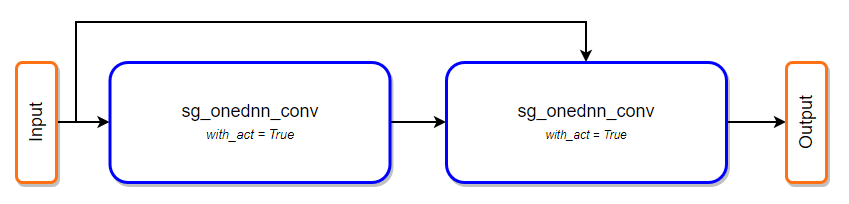
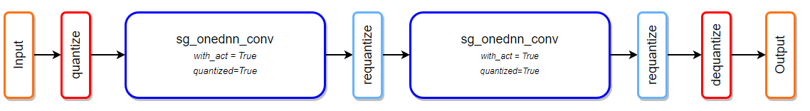
Firstly quantization performs operator fusion on floating-point model as
mentioned in paragraph earlier. Next, all operators which support int8 data
type are marked as quantized and if needed additional operators are injected
into graph surrounding quantizable operator - the goal of this additional
operators is to quantize, dequantize or requantize data to keep data type
between operators compatible.
-
+
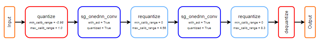
-After injection step it is important to perform calibration of the model,
however this step is optional. Quantizing without calibration is not
recommended in terms of performance. It will result in calculating data minimum
and maximum in quantize and requantize nodes during each inference pass.
Calibrating a model greatly improves performance as minimum and maximum values
are collected offline and are saved inside node - this way there is no need to
search for these values during inferen [...]
+After injection step it is important to perform calibration of the model,
however this step is optional. Quantizing without calibration is not
recommended in terms of performance. It will result in calculating data minimum
and maximum in quantize and requantize nodes during each inference pass.
Calibrating a model greatly improves performance as minimum and maximum values
are collected offline and are saved inside node - this way there is no need to
search for these values during inferen [...]
@@ -142,6 +142,7 @@ net = resnet50_v1(pretrained=True)
```
Now, to get a ready-to-deploy quantized model two steps are required:
+
1. Prepare data loader with calibration data - this data will be used as input
to the network. All necessary layers will be observed with layer collector to
calculate minimum and maximum value of that layer. This flow is internal
mechanism and all what user needs to do is to provide data loader.
2. Call `quantize_net` function from `contrib.quantize` package - both
operator fusion calls will be called inside this API.
@@ -156,19 +157,19 @@ Following function, which calculates total inference time
on the model with an a
def benchmark_net(net, batch_size=32, batches=100, warmup_batches=5):
import time
data = mx.np.random.uniform(-1.0, 1.0, (batch_size, 3, 224, 224))
-
+
for i in range(batches + warmup_batches):
if i == warmup_batches:
tic = time.time()
out = net(data)
out.wait_to_read()
-
+
total_time = time.time() - tic
return total_time
```
-Comparing fused float32 network to quantized network on CLX8280 shows 4.29x
speedup - measurment was done on 28 cores and this machine utilizes VNNI
instruction set.
+Comparing fused float32 network to quantized network on Intel(R) Xeon(R)
Platinum 8375C CPU shows *4.2x speedup* - measurment was done on 32 cores and
this machine utilizes VNNI instruction set.
The other aspect of lowering the precision of a model is a difference in its
accuracy. We will check that on previously tested resnet50_v1 with ImageNet
dataset. To run this example you will need ImageNet dataset prepared with this
tutorial and stored in path_to_imagenet. Let’s compare top1 and top5 accuracy
of standard fp32 model with quantized int8 model calibrated using naive and
entropy calibration mode. We will use only 10 batches of the validation dataset
to calibrate quantized model.
@@ -179,24 +180,26 @@ from mxnet.gluon.model_zoo.vision import resnet50_v1
from mxnet.gluon.data.vision import transforms
from mxnet.contrib.quantization import quantize_net
-def test_accuracy(net, data_loader):
+def test_accuracy(net, data_loader, description):
acc_top1 = mx.gluon.metric.Accuracy()
acc_top5 = mx.gluon.metric.TopKAccuracy(5)
-
+ count = 0
+ tic = time.time()
for x, label in data_loader:
+ count += 1
output = net(x)
acc_top1.update(label, output)
acc_top5.update(label, output)
-
+ time_spend = time.time() - tic
_, top1 = acc_top1.get()
_, top5 = acc_top5.get()
+ print('{:12} Top1 Accuracy: {:.4f} Top5 Accuracy: {:.4f} from {:4} batches
in {:8.2f}s'
+ .format(description, top1, top5, count, time_spend))
- return top1, top5
-
rgb_mean = (0.485, 0.456, 0.406)
rgb_std = (0.229, 0.224, 0.225)
batch_size = 64
-
+
dataset = mx.gluon.data.vision.ImageRecordDataset('path_to_imagenet/val.rec')
transformer = transforms.Compose([transforms.Resize(256),
transforms.CenterCrop(224),
@@ -205,31 +208,33 @@ transformer = transforms.Compose([transforms.Resize(256),
val_data = mx.gluon.data.DataLoader(dataset.transform_first(transformer),
batch_size, shuffle=True)
net = resnet50_v1(pretrained=True)
-net.hybridize(backend='ONEDNN', static_alloc=True, static_shape=True)
+net.hybridize(static_alloc=True, static_shape=True)
+test_accuracy(net, val_data, "FP32")
-top1, top5 = test_accuracy(net, val_data)
-print('FP32 Top1 Accuracy: {} Top5 Accuracy: {}'.format(top1, top5))
+dummy_data = mx.np.random.uniform(-1.0, 1.0, (batch_size, 3, 224, 224))
+net.optimize_for(dummy_data, backend='ONEDNN', static_alloc=True,
static_shape=True)
+test_accuracy(net, val_data, "FP32 fused")
qnet = quantize_net(net, calib_mode='naive', calib_data=val_data,
num_calib_batches=10)
qnet.hybridize(static_alloc=True, static_shape=True)
-top1, top5 = test_accuracy(qnet, val_data)
-print('INT8Naive Top1 Accuracy: {} Top5 Accuracy: {}'.format(top1, top5))
+test_accuracy(qnet, val_data, 'INT8 Naive')
qnet = quantize_net(net, calib_mode='entropy', calib_data=val_data,
num_calib_batches=10)
qnet.hybridize(static_alloc=True, static_shape=True)
-top1, top5 = test_accuracy(qnet, val_data)
-print('INT8Entropy Top1 Accuracy: {} Top5 Accuracy: {}'.format(top1, top5))
+test_accuracy(qnet, val_data, 'INT8 Entropy')
```
#### Output:
-> FP32 Top1 Accuracy: 0.76364 Top5 Accuracy: 0.93094
-> INT8Naive Top1 Accuracy: 0.76028 Top5 Accuracy: 0.92796
-> INT8Entropy Top1 Accuracy: 0.76404 Top5 Accuracy: 0.93042
+> ``FP32 Top1 Accuracy: 0.7636 Top5 Accuracy: 0.9309 from 782 batches
in 1560.97s``
+> ``FP32 fused Top1 Accuracy: 0.7636 Top5 Accuracy: 0.9309 from 782 batches
in 281.03s``
+> ``INT8 Naive Top1 Accuracy: 0.7631 Top5 Accuracy: 0.9309 from 782 batches
in 184.87s``
+> ``INT8 Entropy Top1 Accuracy: 0.7617 Top5 Accuracy: 0.9298 from 782 batches
in 185.23s``
+
With quantized model there is a tiny accuracy drop, however this is the cost
of great performance optimization and memory footprint reduction. The
difference between calibration methods is dependent on the model itself, used
activation layers and the size of calibration data.
### Custom layer collectors and calibrating the model
-In MXNet 2.0 new interface for creating custom calibration collector has been
added. Main goal of this interface is to give the user as much flexibility as
possible in almost every step of quantization. Creating own layer collector is
pretty easy, however computing effective min/max values can be not a trivial
task.
+In MXNet 2.0 new interface for creating custom calibration collector has been
added. Main goal of this interface is to give the user as much flexibility as
possible in almost every step of quantization. Creating own layer collector is
pretty easy, however computing effective min/max values can be not a trivial
task.
Layer collectors are responsible for collecting statistics of each node in the
graph — it means that the input/output data of every operator executed can be
observed. Collector utilizes the register_op_hook method of HybridBlock class.
@@ -244,27 +249,27 @@ class ExampleNaiveCollector(CalibrationCollector):
# important! initialize base class attributes
super(ExampleNaiveCollector, self).__init__()
self.logger = logger
-
+
def collect(self, name, op_name, arr):
"""Callback function for collecting min and max values from an NDArray."""
if name not in self.include_layers: # include_layers is populated by
quantization API
return
arr = arr.copyto(cpu()).asnumpy()
-
+
min_range = np.min(arr)
max_range = np.max(arr)
-
+
if name in self.min_max_dict: # min_max_dict is by default empty dict
cur_min_max = self.min_max_dict[name]
self.min_max_dict[name] = (min(cur_min_max[0], min_range),
max(cur_min_max[1], max_range))
else:
self.min_max_dict[name] = (min_range, max_range)
-
+
if self.logger:
self.logger.debug("Collecting layer %s min_range=%f, max_range=%f"
% (name, min_range, max_range))
-
+
def post_collect(self):
# we're using min_max_dict and don't process any collected statistics so we
don't
# need to override this function, however we are doing this for the sake of
this article
@@ -278,7 +283,7 @@ After collecting all statistic data post_collect function
is called. In post_col
```
from mxnet.contrib.quantization import *
import logging
-logging.basicConfig(level=logging.DEBUG)
+logging.getLogger().setLevel(logging.DEBUG)
#…
@@ -293,13 +298,15 @@ qnet = quantize_net(net, calib_mode='custom',
calib_data=calib_data_loader, Laye
### Performance
Performance results of CV models. Chart presents three different runs: base
float32 model without optimizations, fused float32 model with optimizations and
quantized model.
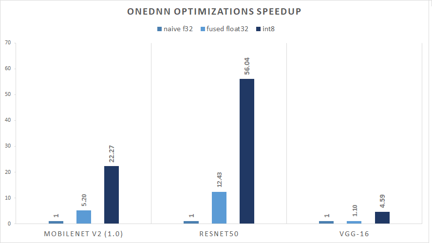
-###### Relative Inference Performance (img/sec) for Batch Size 128
+**Figure 1.** Relative Inference Performance (img/sec) for Batch Size 128
### Accuracy
Accuracy results of CV models. Chart presents three different runs: base
float32 model without optimizations, fused float32 model with optimizations and
fused quantized model.
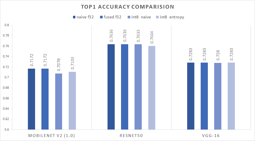
-###### ImageNet(ILSVRC2012) TOP1 validation accuracy
+**Figure 2.** ImageNet(ILSVRC2012) TOP1 validation accuracy
## Notes
-- Accuracy and speedup tested on AWS c6i.16xlarge
-- MXNet SHA: 9fa75b470b8f0238a98635f20f5af941feb60929 / oneDNN SHA:
f40443c413429c29570acd6cf5e3d1343cf647b4
\ No newline at end of file
+Accuracy and speedup tested on:
+- AWS c6i.16xlarge EC2 instance with Ubuntu 20.04 LTS (ami-0558cee5b20db1f9c)
+- MXNet SHA: 9fa75b470b8f0238a98635f20f5af941feb60929 / oneDNN v2.6 SHA:
52b5f107dd9cf10910aaa19cb47f3abf9b349815
+- with following enviroment variables were set: ``OMP_NUM_THREADS=32
OMP_PROC_BIND=TRUE OMP_PLACES={0}:32:1`` (by
[benchmark/python/dnnl/run.sh](https://github.com/apache/incubator-mxnet/blob/102388a0557c530741ed8e9b31296416a1c23925/benchmark/python/dnnl/run.sh))