Hi Justin,
regarding K and epsilon: K is actually an initial setting of section size and
it should be equal to Theta(1 / epsilon), regardless of the stream length SL.
This is because SL is not known in advance and we maintain the correct section
size dynamically. That is, each compactor starts assuming that SL is small
(i.e. SL = O(K)), so it has just 3 sections of size K, and every time the
number of sections needs to be increased because (# of compactions) > 2^(# of
sections), we decrease K by a factor of sqrt(2) for that compactor and double
the number of sections.
So, it seems to me that in the implementation, the relation between K and
\varepsilon is quite clear, up to a constant factor :-) The relation of K and
epsilon is only complicated in the paper, where we involve SL in the definition
of K.
Pavel
PS: I agree that we should have more samples of the error distribution towards
the tail that we care about
On 2020-09-14 14:32, Justin Thaler wrote:
> that's fine, but 64 points over the entire range means we haven't actually
> confirmed that it's working properly as you approach the tail. It's not
> sampled well enough at the tails to observe that behavior.
I'll second that the primary motivation behind studying relative-error
quantiles is to get really good accuracy in the tail. So while we should, of
course, carefully characterize the error behavior over the whole range of
ranks, a key component of the characterization should be to understand in
practice how the error is behaving in the tail. This may require significantly
more fine-grained characterization testing in the tail than we are used to.
In particular, a lot of the ongoing discussion may just stem from the fact that
the quantiles being reported are just the integer multiples of 1/64. My initial
reaction is that the benefit of the relative-error sketch will be more apparent
if the characterization tests cut up the interval [0, 1/64] much more finely.
For example, the theory guarantees that for Low-Rank-Accuracy, items of
(absolute) rank 0, 1, ..., 1/\varepsilon have exact counts, items of rank
(1/\varepsilon)+1, (1/\varepsilon)+2, ..., 2\varepsilon have absolute error at
most 1, and so on.
In terms of relative ranks (normalized by stream length SL), each interval of
1/\varepsilon items referenced above has length just \varepsilon/SL, i.e., we
only guarantee exact counts for items of relative rank [0, \varepsilon/SL].
If \varepsilon is, say, 0.01, and SL is 2^{17}, then we are talking about
intervals of length less than 0.001. This means that I am not surprised to see
that we do not get _exact_ counts out of the sketch in practice even in the
tail if we are effectively defining the tail to be all items of relative rank
[0, 1/64]~=[0, 0.015].
It's a bit tricky to try to figure out what setting of \varepsilon is
(implicitly) being used in the current characterization code since the
parameter provided is K as opposed to \varepsilon.
I think K here means each buffer of size ~2B is viewed by the algorithm as
consisting of 2B/K blocks of length K. In which case, if I recall correctly,
the paper wants to set K to Theta((1/\varepsilon)/\sqrt{log_2(\varepsilon
*SL)}) (with complications arising because SL is not known in advance, and with
sizeable constants hidden by the Big-Theta-notation), see Equation 16 of
https://arxiv.org/pdf/2004.01668.pdf. So in principle, once you tell me SL, I
can probably derive the value of \varepsilon corresponding to any value of K,
but this is complicated in practice since the expression defining K in terms of
\varepsilon and SL is complicated.
This is not any sort of criticism of the information that Lee has provided :-).
It is just an inherently annoying thing to relate K to the \varepsilon
parameter appearing in the theoretical analysis of the algorithm.
On Mon, Sep 14, 2020 at 3:19 AM Jon Malkin
<[email protected]<mailto:[email protected]>> wrote:
If you want to also test the whole range, that's fine, but 64 points over the
entire range means we haven't actually confirmed that it's working properly as
you approach the tail. It's not sampled well enough at the tails to observe
that behavior.
Ok, first off, this is what the original quantiles sketch does to solve
equations going above 1.0/below 0.0:
https://github.com/apache/incubator-datasketches-java/blob/master/src/main/java/org/apache/datasketches/quantiles/DoublesSketch.java#L240
https://github.com/apache/incubator-datasketches-java/blob/master/src/main/java/org/apache/datasketches/quantiles/DoublesSketch.java#L251
In other words, we just clip the result to stay within the known range. Because
the raw formula doesn't care about such limits and will happily return
something outside that range otherwise.
And our existing bounds on the classic quantiles sketch are too pessimistic
most of the time. I mean take this simple code example:
public void rankErrorTest() {
int n = 1 << 20;
int k = 1 << 5;
UpdateDoublesSketch sketch = DoublesSketch.builder().setK(k).build();
for (int i = 0; i < n-1; i++)
sketch.update(rand.nextGaussian());
System.err.println("Retained: " + sketch.getRetainedItems() + "\tNormRakErr:
" + sketch.getNormalizedRankError(false));
sketch.update(rand.nextGaussian());
System.err.println("Retained: " + sketch.getRetainedItems() + "\tNormRakErr:
" + sketch.getNormalizedRankError(false));
}
I insert n-1 items, then print retained items and rank error. Then I insert 1
more and do the same. The output is:
Retained: 511 NormRakErr: 0.05415609535374165
Retained: 32 NormRakErr: 0.05415609535374165
And that makes sense since our rank error function doesn't take into account n
at all. As a result, we have no better an error estimate when retaining 511
items compared to 32. The error bound is clearly being overly conservative, not
taking advantage of how many items we're actually retaining. It's the 99th
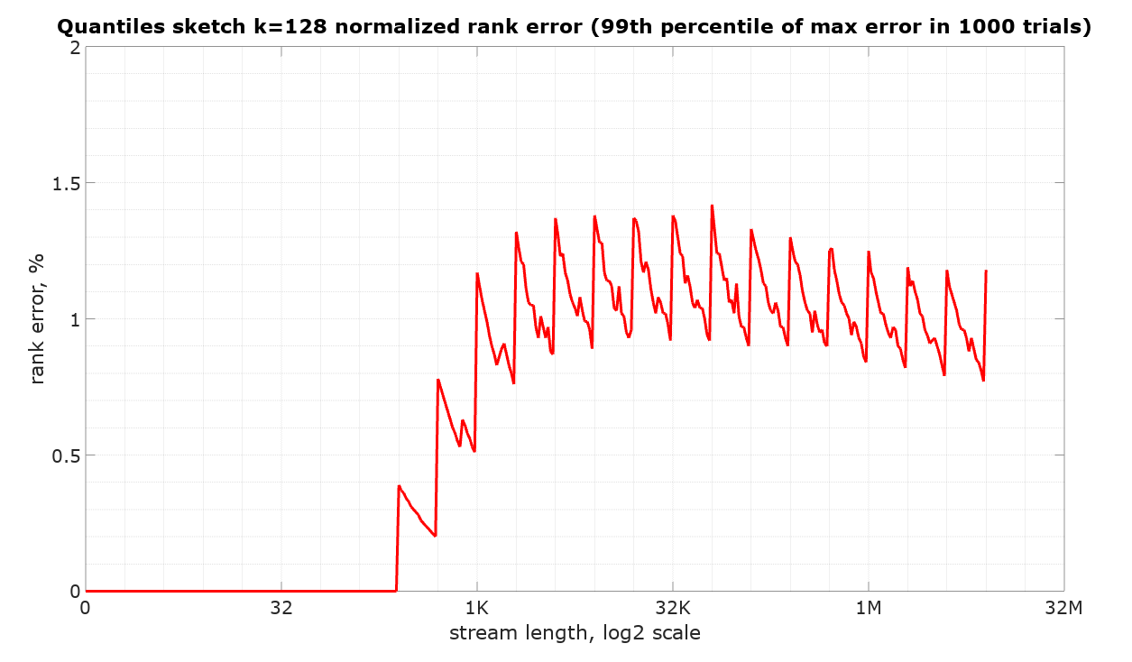
percentile plot, but we see this in our documentation here:
http://datasketches.apache.org/docs/img/quantiles/qds-7-compact-accuracy-1k-99pct-20180224.png
With the error guarantee in the paper of |\hat{R}(y) - R(y)| <= \varepsilon
R(y), the linear bounds seems correct. In fact, anything with error increasing
exponentially seems suspiciously odd. But perhaps I didn't think through the
details of the rank definition enough.
Anyway, maybe I'm just confused by what exactly you mean by "predict the actual
error behavior"?
jon
On Sun, Sep 13, 2020, 10:02 PM leerho
<[email protected]<mailto:[email protected]>> wrote:
I disagree. The bounds on our current sketches do a pretty good job of
predicting the actual error behavior. That is why we have gone to the trouble
of allowing the user to choose the size of the confidence interval and in the
case of the theta Sketches we actually track the growth of the error Contour in
the early stages of Estimation mode. The better we can specify the error, the
more confident the user will be in the result.
For these early characterization tests it is critical to understand the error
behavior over the entire range of ranks. How we ultimately specify and
document how to properly use this sketch we will do later.
Lee.
On Sun, Sep 13, 2020 at 1:45 PM Jon Malkin
<[email protected]<mailto:[email protected]>> wrote:
Our existing bounds, especially for the original quantities sketch, don't
necessarily predict the actual error behavior. They're an upper bound on it.
Especially right before one of the major cascading compaction rounds, our error
may be substantially better than the bound.
I also feel like characterization plots going from 0.0-1.0 kind of misses the
point of the relative error quantiles sketch. It's kind of useful to know what
it's doing everywhere but if you care about that whole range you should be
using KLL, not this sketch. If you care about accuracy over the whole range and
also high precision at the tail, you should be using both sketches together.
The interesting thing with this sketch would be to focus only on error in, say,
the outer 5% at most. Maybe even a log scale plot approaching the edge of the
range.
jon
--
From my cell phone.