You're right that microbenchmarks often do not reflect real-world
performance, but in defense of using the sample mean for benchmarking, it's
a good estimator of the population mean (provided the distribution has
finite variance), and if you perform an operation n times, it will take
about nμ seconds. If you want your code to run as fast as possible that's
probably what matters.
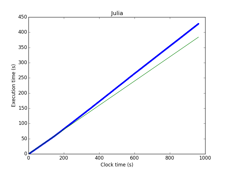
The reason Julia's behavior is periodic and Octave's is not is almost
certainly Octave uses reference counting, which incurs overhead whenever an
array is allocated or destroyed, while Julia uses garbage collection, which
incurs overhead only once a certain amount of memory has been allocated.
People are certainly aware that Julia's garbage collector is suboptimal
<https://github.com/JuliaLang/julia/issues/261>, and there is work being
done <https://github.com/JuliaLang/julia/pull/5227> to improve it. As long
as you run an operation enough times, the mean will accurately reflect
garbage collection overhead. (That isn't just by chance.) But the frequency
of garbage collection will depend not only on the amount of memory
allocated, but also on the total amount of memory the system has, so that
is not necessarily useful unless you benchmark on the same machine.

Simon

On Friday, September 12, 2014 11:11:13 AM UTC-4, [email protected] wrote:
>
> A few days ago, Ján Dolinský posted some microbenchmark
> <https://groups.google.com/d/topic/julia-users/n3LfteWJAd4/discussion>s
> about Julia being slower than Octave for squaring quite large matrices. At
> that time, I wanted to answer with the traditional *microbenchmarks are
> evil*™ type of answer.
>
> I wanted to emphases that:
>
>    1. The mean is hardly a good distribution location estimator in the
>    general (non-normal) case.
>    2. Neglecting that, what he calculated was a typical execution time
>    for the squaring of *one and only one* random matrix filled with
>    7000x7000 random Float64 numbers with his computer.
>    3. Assuming the 7000x7000 matrix size represents the typical matrix
>    size for his work, that means that Julia is likely *fast enough*: it's
>    bellow 1 s, the difference between Julia and Octave is not noticeable by
>    anything except a computer.
>
>
> But from his latter concerns, I guess this was not really what he had in
> mind (but I may have misinterpreted his words). I supposed that what he
> really wanted was to calculate *many *of such squared matrices, so many
> of them that the observed difference in execution times would matter a lot.
>
>
> What would be a not-too-bad benchmark adapted to this use case? I guess
> repeating the calculation is required. But instead of measuring time
> outside of the loop, it might be very interesting to get it inside of the
> loop: for each one of the squarings. These individual measurements, if not
> too short, would allow us:
>
>    - to plot the complete time distribution instead of assuming normality
>    and providing only one distribution parameter;
>    - to get the cumulative distribution to represent the case of multiple
>    consecutive matrix squarings;
>    - to follow the execution time evolution through time or iterations.
>
> So here is the snippet of code that I used:
>
> t = Float64[]
> for i = 1:2020
>     X = rand(1000,1000)
>     tic()
>         XX = X.^2
>     b = toq()
>     push!(t, b)
> end
>
> The matrix generation is in-loop to avoid any smart caching.
>
>
> *1- Distributions*
>
> So here are the distributions (mind the Y axis is log):
>
>
> <https://lh5.googleusercontent.com/-9FN8ZPU-0pc/VBMAGn_zEyI/AAAAAAAAABo/4LgTyyxCATk/s1600/1-Distributions.png>
>
> Octave execution times are small and very close from each other. The
> behavior of those two Julia repetitions of the same calculation are much
> weirder : there is not just one peak, but 3 or 4. That's a strong hint
> *against* mean calculations. Furthermore, complete distributions contain
> much more information. I really think that calculating such estimations of
> the distributions is the bare minimum when benchmarking.
>
> Ooops, I just said it: *estimations*. The methods used to estimate
> distributions usually need arbitrary parameters to be set (here, the
> Gaussian kernel and its bandwidth). So the peaks above are of almost
> arbitrary width. Who do I know whether these peaks represent something or
> are just produced by poor bandwidth choice? Repetitions of the whole
> process is one good way to test that. But here, I'll take another approach:
> plotting execution time vs. the iteration numbers.
>
> *2- Execution times vs. iteration number*
>
> So let's look at these execution times:
>
>
> <https://lh5.googleusercontent.com/-J67l7RmdAG0/VBMAKHyh4uI/AAAAAAAAABw/GwLg8oJUbk0/s1600/2-Execution%2Btimes%2Bvs.%2Biteration%2Bnumber.png>
>
> Ohoh! (Not so) Surprising! While Octave seems to behave as expected
> (random distribution around a single value), Julia exhibits a completely
> different profile: there are 4 different layers. Having done other
> repetitions, Julia's baseline seems to always be more or less the same but
> there are regular execution time bumps now and then. And if you look very
> carefully, you'll see that there is a bump around iteration #1550 in the
> "Julia (rep.)" case. More on that later.
>
> *3- Periodogram*
>
> So I just wanted to have a look at these bumps more carefully. Are they
> always occurring with a given frequency? A good way to answer this question
> is to plot the periodogram:
>
>
> <https://lh5.googleusercontent.com/-bZxkeMbD3Ik/VBMARRz8SVI/AAAAAAAAAB4/VkXtW-q3CPI/s1600/3-Periodogram_0.png>
>
> Julia periodogram shows that the bumps mostly occur every 3 iterations.
> This kind of frequency dependency is not exhibited by Octave.
>
> From there, I don't really know how to go a lot further than that:
> profiling may help and since @time has the capability to distinguish
> between calculation- and GC-related execution times, I guess it wouldn't be
> so hard to look into this from a GC perspective. This behaviour can also be
> clearly seen in some parts of the Time(iteration #) graph:
>
>
> <https://lh6.googleusercontent.com/-qssnaM10bXQ/VBMAUAzCBMI/AAAAAAAAACA/OA5GAJyPNj4/s1600/3-Periodogram_1.png>
> How is that important? Things like periodicity can give very strong hints
> about what is actually happening. Raw results are not enough and this is
> one reason why most benchmarks are useless. The second reason is that there
> is a discrepancy between the question asked and the answer calculated:
> let's go forward to cumulative density functions.
>
>
> *4- Cumulative density function of execution time*
>
> CDF does actually represent the execution time elapsed after a given
> number of iterations. This metric is more interesting than
> single measurements averaging because it does not presuppose normality.
> Here is an example :
>
>
> <https://lh4.googleusercontent.com/-Gz16JMCGr5A/VBMAYEAs2ZI/AAAAAAAAACI/wjprIGyNuEk/s1600/4-Cumulative%2Bdensity%2Bfunction.png>
>
> Dots are actual values. The red line corresponds to the estimated CDF of
> Julia in the case where bumps are avoided. The cyan one corresponds to the
> current case (bumps every 3 or so iterations). By chance, these curves are
> almost linear which means that taking the average of many values is not so
> bad of an approximation. However, no one would ever have noticed that *most
> *(2/3) of the cases are calculated quite quickly while 1/3 of them take 3
> times as much time to be calculated. And I repeat: by chance.
>
>
> *5- Conclusion*
>
> Are we finished yet? Of course not. There are so many interactions that
> it's really hard to get a useful insight. I've only scratched the surface.
> Look at this for instance:
>
>
> <https://lh6.googleusercontent.com/-3m3VKUBZ4qI/VBMAbWNpVKI/AAAAAAAAACQ/nPTc1TLvqXc/s1600/5-Conclusion.png>
>
> This is a longer Julia run. I've also recorded CPU and RAM usage at the
> same time: no correlation at all. But there seems to be an OS- or
> Julia-related long term effect on the calculations. Transform that to a CDF
> and you'll see that our naive curve of part 4 is only really the tip of the
> iceberg:
>
>
> <https://lh4.googleusercontent.com/-geSdEeNdIZc/VBMLLob-bGI/AAAAAAAAACc/-2kehcTrCgo/s1600/5-conclusion_2.png>
> Depending on where you calculated your average, you are likely to
> overestimate or to underestimate the actual execution time by a large
> margin. This curve is an example of microbenchmarking failure. Benchmarking
> is useless: profile complete programs instead.
>
>
> My purpose was really not to prove anything performance-wise (both Julia
> and Octave code were* not* optimized). This was not the point.
> I just wanted:
>
>    1.  to show that it's already very complicated to get meaningful
>    results on *one's* computer, in *one's* use case, for *one's*
>    particular calculation with all these efforts to set the problem correctly;
>    2. to make sure that these periodic behaviours are expected by Julia
>    devs and known.
>
>
> So, at least, as a simple reader on these forums, I would be very very
> very pleased if we could provide at least histograms of execution time
> distributions instead of just giving one raw number. This won't tell a lot
> more, but it can make the difference.
>