The dominant source of error in an intensity measurement actually
depends on the magnitude of the intensity. For intensities near zero
and with zero background, the "read-out noise" of image plate or
CCD-based detectors becomes important. On most modern CCD detectors,
however, the read-out noise is quite low: equivalent to the noise
induced by having only a few "extra" photons/pixel (if any). For
intensities of more than ~1000 photons, the calibration of the detector
(~2-3% error) starts to dominate. It is only for a "midrange" between
~2 photons/pixel and 1000 integrated photons that "shot noise" (aka
"photon counting error" or "Poisson statistics") plays the major role.
So it is perhaps a bit ironic that the "photon counting error" we worry
so much about is only significant for a very narrow range of intensities
in any given data set.
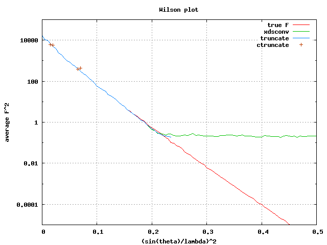
But yes, there does seem to be something "wrong" with ctruncate. It can
throw out a great deal of hkls that both xdsconv and the "old truncate"
keep. Graph of the resulting Wilson plots here:
http://bl831.als.lbl.gov/~jamesh/bugreports/ctruncate/truncated_wilsons.png
and the script for producing the data for this plot from "scratch":
http://bl831.als.lbl.gov/~jamesh/bugreports/ctruncate/truncate_notes.com
Note that only 3 bins are even populated in the ctruncate result,
whereas "truncate" and "xdsconv" seem to reproduce the true Wilson plot
faithfully down to well below the noise, which in this case is a
Gaussian deviate with RMS = 1.0 added to each F^2.
The "plateau" in the result from xdsconv is something I've been working
with Kay to understand, but it seems to be a problem with the
French-Wilson algorithm itself, and not any particular implementation of
it. Basically, French and Wilson did not want to assume that the Wilson
plot was straight and therefore don't use the "prior information" that
if the intensities dropped into the noise at 2.0 A then the average
value of "F" and 1.0 A is much much less than "sigma"! As a result, the
French-Wilson values for "F" far above the traditional "resolution
limit" can be overestimated by as much as a factor of a million.
Perhaps this is why truncate and ctruncate complain bitterly about "data
beyond useful resolution limit".
A shame really, because if the Wilson plot of the "truncated" data is
made to follow the linear trend we see in the low-angle data, then we
wouldn't need to argue so much. After all, the only reason we apply a
resolution cutoff is to try and suppress the "noise" coming from all
those background-only spots at high angle. But, on the other hand, we
don't want to cut the data too harshly or we will get series-termination
errors. So, we must strike a compromise between these two sources of
error and call that the "resolution cutoff". But, if the conversion of
I to F actually used the "prior knowledge" of the fall-off of the Wilson
plot with resolution, then there would be no need for a "resolution
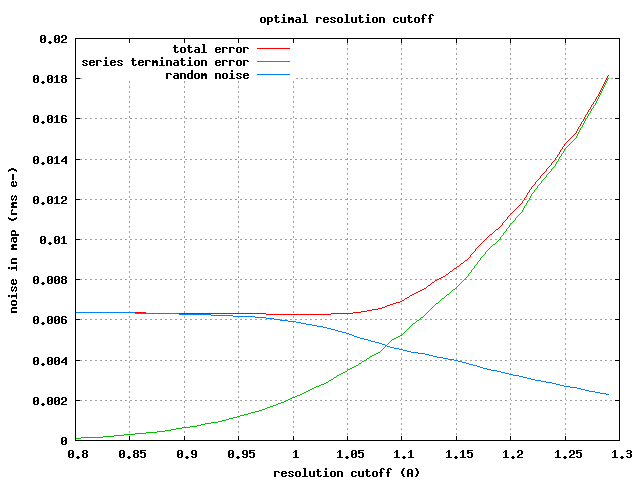
cutoff" at all. The current situation is portrayed in this graph:
http://bl831.als.lbl.gov/~jamesh/wilson/error_breakdown.png
which just showed the noise induced in an electron density map by
applying a resolution cutoff to otherwise "perfect" data, vs the error
due to adding noise and running truncate. If the noisy data were
down-weighted only a little bit, then the "total noise" curve would
continue to drop, even at "infinite resolution".
I think it is also important to point out here that the "resolution
cutoff" of the data you provide to refmac or phenix.refine is not
necessarily the "resolution of the structure". This latter quantity,
although emotionally charged, really does need to be more well-defined
by this community and preferably in a way that is historically
"stable". You can't just take data that goes to 5.0A and call it "4.5A
data" by changing your criterion. Yes, it is "better" to refine out to
4.5A when the intensities drop into the noise at 5A, but that is never
going to be as good as using data that does not drop into the noise
until 4.5A.
-James Holton
MAD Scientist

On 6/27/2013 9:30 AM, Ian Tickle wrote:
On 22 June 2013 19:39, Douglas Theobald <[email protected]
<mailto:[email protected]>> wrote:
    So I'm no detector expert by any means, but I have been assured by
    those who are that there are non-Poissonian sources of noise --- I
    believe mostly in the readout, when photon counts get amplified.
     Of course this will depend on the exact type of detector, maybe
    the newest have only Poisson noise.
Sorry for delay in responding, I've been thinking about it. It's
indeed possible that the older detectors had non-Poissonian noise as
you say, but AFAIK all detectors return _unsigned_ integers (unless
possibly the number is to be interpreted as a flag to indicate some
error condition, but then obviously you wouldn't interpret it as a
count). So whatever the detector AFAIK it's physically impossible for
it to return a negative number that is to be interpreted as a photon
count (of course the integration program may interpret the count as a
_signed_ integer but that's purely a technical software issue). I
think we're all at least agreed that, whatever the true distribution
of Ispot (and Iback) is, it's not in general Gaussian, except as an
approximation in the limit of large Ispot and Iback (with the proviso
that under this approximation Ispot & Iback can never be negative).
Certainly the assumption (again AFAIK) has always been that var(count)
= count and I think I'm right in saying that only a Poisson
distribution has that property?
    No, its just terminology.  For you, Iobs is defined as
    Ispot-Iback, and that's fine.  (As an aside, assuming the Poisson
    model, this Iobs will have a Skellam distribution, which can take
    negative values and asymptotically approaches a Gaussian.)  The
    photons contributed to Ispot from Itrue will still be Poisson.
     Let's call them something besides Iobs, how about Ireal?  Then,
    the Poisson model is

    Ispot = Ireal + Iback'

    where Ireal comes from a Poisson with mean Itrue, and Iback' comes
    from a Poisson with mean Iback_true.  The same likelihood function
    follows, as well as the same points.  You're correct that we can't
    directly estimate Iback', but I assume that Iback (the counts
    around the spot) come from the same Poisson with mean Iback_true
    (as usual).

    So I would say, sure, you have defined Iobs, and it has a Skellam
    distribution, but what, if anything, does that Iobs have to do
    with Itrue?  My point still holds, that your Iobs is not a valid
    estimate of Itrue when Ispot<Iback.  Iobs as an estimate of Itrue
    requires unphysical assumptions, namely that photon counts can be
    negative.  It is impossible to derive Ispot-Iback as an estimate
    for Itrue (when Ispot<Iback) *unless* you make that unphysical
    assumption (like the Gaussian model).
Please note that I have never claimed that Iobs = Ispot - Iback is to
be interpreted as an estimate of Itrue, indeed quite the opposite: I
agree completely that Iobs has little to do with Itrue when Iobs is
negative. In fact I don't believe anyone else is claiming that Iobs
is to be interpreted as an estimate of Itrue either, so maybe this is
the source of the misunderstanding? Certainly for me Ispot - Iback is
merely the difference between the two measurements, nothing more.
Maybe if we called it something other than Iobs (say Idiff), or even
avoided giving it a name altogether that would avoid any further
confusion? Perhaps this whole discussion has been merely about
terminology?
    I'm also puzzled as to your claim that Iback' is not Poisson.  I
    don't think your QM argument is relevant, since we can imagine
    what we would have detected at the spot if we'd blocked the
    reflection, and that # of photon counts would be Poisson.  That is
    precisely the conventional logic behind estimating Iback' with
    Iback (from around the spot), it's supposedly a reasonable
    control.  It doesn't matter that in reality the photons are
    indistinguishable --- that's exactly what the probability model is
    for.
I'm not clear how you would "block the reflection"? How could you do
that without also blocking the background under it? A large part of
the background comes from the TDS which is coming from the same place
that the Bragg diffraction is coming from, i.e. the crystal. I know
of no way of stopping the Bragg diffraction without also stopping the
TDS (or vice versa). Indeed the theory shows that there is in reality
no distinction between Bragg diffraction and TDS; they are just
components of the total scattering that we find convenient to imagine
as separate in the dynamical model of scattering (see
http://people.cryst.bbk.ac.uk/~tickle/iucr99/s61.html
<http://people.cryst.bbk.ac.uk/%7Etickle/iucr99/s61.html> for the
relevant equations).
Any given photon "experiences" the whole crystal on its way from the
source to the detector (in fact it experiences more than that: it
traverses all possible trajectories simultaneously, it's just that the
vast majority cancel by destructive interference). The resulting wave
function of the photon only collapses to a single point on hitting the
detector, with a frequency proportional to the square of the wave
function at that point, so it's meaningless to talk about the
trajectory of an individual photon or whether it "belongs" to Ireal or
Iback'. You can't talk about the error distribution of the
experimental measurements of some quantity if it's a physical
impossibility to design an experiment to measure it! It can of course
have a probability distribution derived from prior knowledge of the
properties of crystals, but that's not a Poisson, it's a Wilson
(exponential) distribution. Is that what you're thinking of?
According to QM the only real quantities are the observables (or
functions of observables); in this case only Ispot, Iback and
Ispot-Iback (and any other functions of Ispot & Iback that might be
relevant) are physically meaningful quantities, all else is mere
speculation, i.e. part of the model.
As I understand it the reason you are suggesting an alternate way of
estimating Itrue is that you have a fundamental objection to the F & W
algorithm? However I'm not clear precisely what you find
objectionable? Perhaps it would be useful to go through F & W in
detail and identify where the problem (if any) lies?
We can say that the total likelihood of J (= Itrue) given Is (= Ispot)
and Ib (= Iback) is equal to the prior probability density of J given
only knowledge of the crystal (i.e. the estimated no of atoms from
which we can calculate E(J)), multiplied by the joint probability
density of Is and Ib given J and its SD (assumed equal to the SD of
Is-Ib):
P(J | Is,Ib) = P(J | E(J)) P(Is,Ib | J,sdJ)
The only function of Is and Ib that's relevant to the joint
distribution of Is and Ib given J and sdJ, P(Is,Ib | J), is the
difference Is-Ib (at least for large Is and Ib: I don't know what
happens if they are small). Note that it's perfectly proper to talk
about P(Is-Ib | J) in this context: it's the distribution of the
difference you expect to observe given any J. So the above can be
rewritten as:
P(J | Is-Ib) = P(J | E(J)) P(Is-Ib | J,sdJ)
P(Is-Ib | J,sdJ) is just the Gaussian error distribution of Is-Ib
making use of the Gaussian approximation of the Poisson. Finally,
integrating out J to get the expectation of J (or of F=sqrt(J))
completes the F-W procedure. As indicated earlier there are good
reasons to postpone this until after merging equivalents (which is
exactly what we do now).
So what's wrong with that?

Cheers

-- Ian