James answer seems right, and make abject sense. -and makes sense by experience
too..
Bob
Robert Stroud
[email protected]
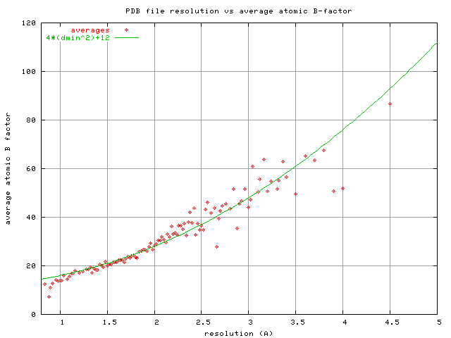
> On Mar 7, 2020, at 12:01 PM, James Holton <[email protected]> wrote:
>
> Yes, that's right.  Model B factors are fit to the data.  That Boverall gets
> added to all atomic B factors in the model before the structure is written
> out, yes?
>
> The best estimate we have of the "true" B factor is the model B factors we
> get at the end of refinement, once everything is converged, after we have
> done all the building we can.  It is this "true B factor" that is a property
> of the data, not the model, and it has the relationship to resolution and map
> appearance that I describe below.  Does that make sense?
>
> -James Holton
> MAD Scientist
>
> On 3/7/2020 10:45 AM, dusan turk wrote:
>> James,
>>
>> The case you’ve chosen is not a good illustration of the relationship
>> between atomic B and resolution.   The problem is that during scaling of
>> Fcalc to Fobs also B-factor difference between the two sets of numbers is
>> minimized. In the simplest form  with two constants Koverall and Boverall it
>> looks like this:
>>
>> sum_to_be_minimized = sum (FOBS**2 -  Koverall * FCALC**2 * exp(-1/d**2 *
>> Boverall) )
>>
>> Then one can include bulk solvent correction, anisotripic scaling, … In
>> PHENIX it gets quite complex.
>>
>> Hence, almost regardless of the average model B you will always get the same
>> map, because the “B" of the map will reflect the B of the FOBS.  When all
>> atomic Bs are equal then they are also equal to average B.
>>
>> best, dusan
>>
>>
>>> On 7 Mar 2020, at 01:01, CCP4BB automatic digest system
>>> <[email protected]> wrote:
>>>
>>>> On Thu, 5 Mar 2020 01:11:33 +0100, James Holton <[email protected]> wrote:
>>>>
>>>>> The funny thing is, although we generally regard resolution as a primary
>>>>> indicator of data quality the appearance of a density map at the classic
>>>>> "1-sigma" contour has very little to do with resolution, and everything
>>>>> to do with the B factor.
>>>>>
>>>>> Seriously, try it. Take any structure you like, set all the B factors to
>>>>> 30 with PDBSET, calculate a map with SFALL or phenix.fmodel and have a
>>>>> look at the density of tyrosine (Tyr) side chains.  Even if you
>>>>> calculate structure factors all the way out to 1.0 A the holes in the
>>>>> Tyr rings look exactly the same: just barely starting to form.  This is
>>>>> because the structure factors from atoms with B=30 are essentially zero
>>>>> out at 1.0 A, and adding zeroes does not change the map.  You can adjust
>>>>> the contour level, of course, and solvent content will have some effect
>>>>> on where the "1-sigma" contour lies, but generally B=30 is the point
>>>>> where Tyr side chains start to form their holes.  Traditionally, this is
>>>>> attributed to 1.8A resolution, but it is really at B=30.  The point
>>>>> where waters first start to poke out above the 1-sigma contour is at
>>>>> B=60, despite being generally attributed to d=2.7A.
>>>>>
>>>>> Now, of course, if you cut off this B=30 data at 3.5A then the Tyr side
>>>>> chains become blobs, but that is equivalent to collecting data with the
>>>>> detector way too far away and losing your high-resolution spots off the
>>>>> edges.  I have seen a few people do that, but not usually for a
>>>>> published structure.  Most people fight very hard for those faint,
>>>>> barely-existing high-angle spots.  But why do we do that if the map is
>>>>> going to look the same anyway?  The reason is because resolution and B
>>>>> factors are linked.
>>>>>
>>>>> Resolution is about separation vs width, and the width of the density
>>>>> peak from any atom is set by its B factor.  Yes, atoms have an intrinsic
>>>>> width, but it is very quickly washed out by even modest B factors (B >
>>>>> 10).  This is true for both x-ray and electron form factors. To a very
>>>>> good approximation, the FWHM of C, N and O atoms is given by:
>>>>> FWHM= sqrt(B*log(2))/pi+0.15
>>>>>
>>>>> where "B" is the B factor assigned to the atom and the 0.15 fudge factor
>>>>> accounts for its intrinsic width when B=0.  Now that we know the peak
>>>>> width, we can start to ask if two peaks are "resolved".
>>>>>
>>>>> Start with the classical definition of "resolution" (call it after Airy,
>>>>> Raleigh, Dawes, or whatever famous person you like), but essentially you
>>>>> are asking the question: "how close can two peaks be before they merge
>>>>> into one peak?".  For Gaussian peaks this is 0.849*FWHM. Simple enough.
>>>>> However, when you look at the density of two atoms this far apart you
>>>>> will see the peak is highly oblong. Yes, the density has one maximum,
>>>>> but there are clearly two atoms in there.  It is also pretty obvious the
>>>>> long axis of the peak is the line between the two atoms, and if you fit
>>>>> two round atoms into this peak you recover the distance between them
>>>>> quite accurately.  Are they really not "resolved" if it is so clear
>>>>> where they are?
>>>>>
>>>>> In such cases you usually want to sharpen, as that will make the oblong
>>>>> blob turn into two resolved peaks.  Sharpening reduces the B factor and
>>>>> therefore FWHM of every atom, making the "resolution" (0.849*FWHM) a
>>>>> shorter distance.  So, we have improved resolution with sharpening!  Why
>>>>> don't we always do this?  Well, the reason is because of noise.
>>>>> Sharpening up-weights the noise of high-order Fourier terms and
>>>>> therefore degrades the overall signal-to-noise (SNR) of the map.  This
>>>>> is what I believe Colin would call reduced "contrast".  Of course, since
>>>>> we view maps with a threshold (aka contour) a map with SNR=5 will look
>>>>> almost identical to a map with SNR=500. The "noise floor" is generally
>>>>> well below the 1-sigma threshold, or even the 0-sigma threshold
>>>>> (https://doi.org/10.1073/pnas.1302823110).  As you turn up the
>>>>> sharpening you will see blobs split apart and also see new peaks rising
>>>>> above your map contouring threshold.  Are these new peaks real?  Or are
>>>>> they noise?  That is the difference between SNR=500 and SNR=5,
>>>>> respectively.  The tricky part of sharpening is knowing when you have
>>>>> reached the point where you are introducing more noise than signal.
>>>>> There are some good methods out there, but none of them are perfect.
>>>>>
>>>>> What about filtering out the noise?  An ideal noise suppression filter
>>>>> has the same shape as the signal (I found that in Numerical Recipes),
>>>>> and the shape of the signal from a macromolecule is a Gaussian in
>>>>> reciprocal space (aka straight line on a Wilson plot). This is true, by
>>>>> the way, for both a molecule packed into a crystal or free in solution.
>>>>> So, the ideal noise-suppression filter is simply applying a B factor.
>>>>> Only problem is: sharpening is generally done by applying a negative B
>>>>> factor, so applying a Gaussian blur is equivalent to just not sharpening
>>>>> as much. So, we are back to "optimal sharpening" again.
>>>>>
>>>>> Why not use a filter that is non-Gaussian?  We do this all the time!
>>>>> Cutting off the data at a given resolution (d) is equivalent to blurring
>>>>> the map with this function:
>>>>>
>>>>> kernel_d(r) = 4/3*pi/d**3*sinc3(2*pi*r/d)
>>>>> sinc3(x) = (x==0?1:3*(sin(x)/x-cos(x))/(x*x))
>>>>>
>>>>> where kernel_d(r) is the normalized weight given to a point "r" Angstrom
>>>>> away from the center of each blurring operation, and "sinc3" is the
>>>>> Fourier synthesis of a solid sphere.  That is, if you make an HKL file
>>>>> with all F=1 and PHI=0 out to a resolution d, then effectively all hkls
>>>>> beyond the resolution limit are zero. If you calculate a map with those
>>>>> Fs, you will find the kernel_d(r) function at the origin.  What that
>>>>> means is: by applying a resolution cutoff, you are effectively
>>>>> multiplying your data by this sphere of unit Fs, and since a
>>>>> multiplication in reciprocal space is a convolution in real space, the
>>>>> effect is convoluting (blurring) with kernel_d(x).
>>>>>
>>>>> For comparison, if you apply a B factor, the real-space blurring kernel
>>>>> is this:
>>>>> kernel_B(r) = (4*pi/B)**1.5*exp(-4*pi**2/B*r*r)
>>>>>
>>>>> If you graph these two kernels (format is for gnuplot) you will find
>>>>> that they have the same FWHM whenever B=80*(d/3)**2.  This "rule" is the
>>>>> one I used for my resolution demonstration movie I made back in the late
>>>>> 20th century:
>>>>> https://bl831.als.lbl.gov/~jamesh/movies/index.html#resolution
>>>>>
>>>>> What I did then was set all atomic B factors to B = 80*(d/3)^2 and then
>>>>> cut the resolution at "d".  Seemed sensible at the time.  I suppose I
>>>>> could have used the PDB-wide average atomic B factor reported for
>>>>> structures with resolution "d", which roughly follows:
>>>>> B = 4*d**2+12
>>>>> https://bl831.als.lbl.gov/~jamesh/pickup/reso_vs_avgB.png
>>>>>
>>>>> The reason I didn't use this formula for the movie is because I didn't
>>>>> figure it out until about 10 years later.  These two curves cross at
>>>>> 1.5A, but diverge significantly at poor resolution.  So, which one is
>>>>> right?  It depends on how well you can measure really really faint
>>>>> spots, and we've been getting better at that in recent decades.
>>>>>
>>>>> So, what I'm trying to say here is that just because your data has CC1/2
>>>>> or FSC dropping off to insignificance at 1.8 A doesn't mean you are
>>>>> going to see holes in Tyr side chains.  However, if you measure your
>>>>> weak, high-res data really well (high multiplicity), you might be able
>>>>> to sharpen your way to a much clearer map.
>>>>>
>>>>> -James Holton
>>>>> MAD Scientist
>>>>>
>> ########################################################################
>>
>> To unsubscribe from the CCP4BB list, click the following link:
>> https://www.jiscmail.ac.uk/cgi-bin/webadmin?SUBED1=CCP4BB&A=1
>
> ########################################################################
>
> To unsubscribe from the CCP4BB list, click the following link:
> https://www.jiscmail.ac.uk/cgi-bin/webadmin?SUBED1=CCP4BB&A=1


########################################################################

To unsubscribe from the CCP4BB list, click the following link:
https://www.jiscmail.ac.uk/cgi-bin/webadmin?SUBED1=CCP4BB&A=1